Extending Pascal's Triangle

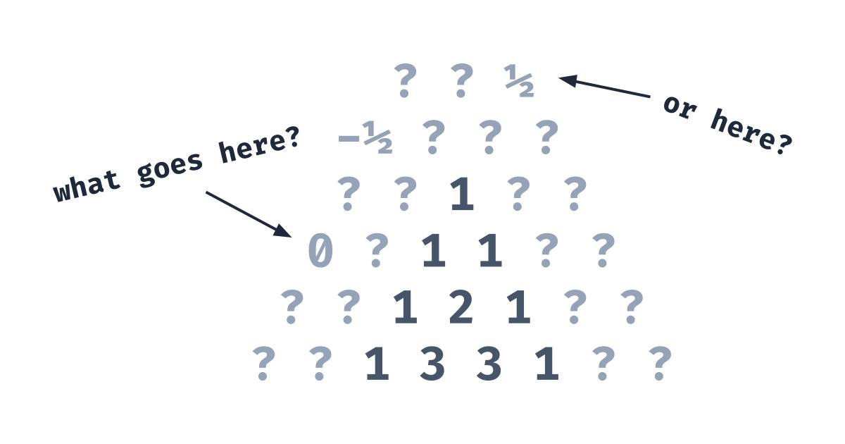
Extending Pascal's triangle beyond its starting point.

Have you heard of Pascal’s Triangle? If so, you’ll know that it can only be extended in a single direction: downward. However, we can use pyramids, factorials, and limits to extend Pascal’s Triangle in the opposite direction. If you haven’t heard of Pascal’s Triangle, you might enjoy this article anyway, and you’ll definitely learn something new.

What is Pascal’s Triangle?

If you already know what Pascal’s Triangle is, you can skip this section. If not, it’s a pretty simple concept to grasp and you’ll be very confused if you skip it.

When making Pascal’s Triangle, start by making a triangle with two diagonals of 11s. In theory, the triangle is limitless, but in practice, it would take a really long time to write that out, so I’ll only include 6 rows.

11111111111\begin{matrix} & & & & & 1 & & & & & \\ & & & & 1 & & 1 & & & & \\ & & & 1 & & & & 1 & & & \\ & & 1 & & & & & & 1 & & \\ & 1 & & & & & & & & 1 & \\ 1 & & & & & & & & & & 1 \\ \end{matrix}

For every cell not on the edge, which should all be 11s, add the cell to the top-left with the cell on the top-right and fill it in. Let’s start with the third row, as the first two are all 11s.

111121111111\begin{matrix} & & & & & 1 & & & & & \\ & & & & 1 & & 1 & & & & \\ & & & 1 & & 2 & & 1 & & & \\ & & 1 & & & & & & 1 & & \\ & 1 & & & & & & & & 1 & \\ 1 & & & & & & & & & & 1 \\ \end{matrix}

That wasn’t very difficult, right? Let’s fill in the fourth row.

11112113311111\begin{matrix} & & & & & 1 & & & & & \\ & & & & 1 & & 1 & & & & \\ & & & 1 & & 2 & & 1 & & & \\ & & 1 & & 3 & & 3 & & 1 & & \\ & 1 & & & & & & & & 1 & \\ 1 & & & & & & & & & & 1 \\ \end{matrix}

I’ll skip to when all six rows are filled in.

11112113311464115101051\begin{matrix} & & & & & 1 & & & & & \\ & & & & 1 & & 1 & & & & \\ & & & 1 & & 2 & & 1 & & & \\ & & 1 & & 3 & & 3 & & 1 & & \\ & 1 & & 4 & & 6 & & 4 & & 1 & \\ 1 & & 5 & & 10 & & 10 & & 5 & & 1 \\ \end{matrix}

Cool! You now know the basics of Pascal’s Triangle.

Special conventions

For the rest of the document, I will use an alternate format to write Pascal’s triangle. The format that uses an actual triangle is difficult to type in LaTeX and hides a few patterns, so we’ll stick to a square shape. This new format provides a more compact version of the original shape, yet it keeps the original patterns. In this shape, we add the cells to the left and above a given item to get its value. Here’s an example:

111111123456136101521141020355615153570126162156126252\begin{matrix} 1 & 1 & 1 & 1 & 1 & 1 & \dots \\ 1 & 2 & 3 & 4 & 5 & 6 & \dots \\ 1 & 3 & 6 & 10 & 15 & 21 & \dots \\ 1 & 4 & 10 & 20 & 35 & 56 & \dots \\ 1 & 5 & 15 & 35 & 70 & 126 & \dots \\ 1 & 6 & 21 & 56 & 126 & 252 & \dots \\ \vdots & \vdots & \vdots & \vdots & \vdots & \vdots & \ddots \\ \end{matrix}

Now that we’ve got that sorted out, let’s get on to the actual content.

All the zeroes

By the rules we’ve defined, if a cell cc has a value, it must be equal to the value of the cell above it, which we’ll call aa, plus the value of the cell to the left of it, which we’ll call bb.

111111123a=45613b=6c=101521141020355615153570126162156126252\begin{matrix} 1 & 1 & 1 & 1 & 1 & 1 & \dots \\ 1 & 2 & 3 & \boxed{a = 4} & 5 & 6 & \dots \\ 1 & 3 & \boxed{b = 6} & \boxed{c = 10} & 15 & 21 & \dots \\ 1 & 4 & 10 & 20 & 35 & 56 & \dots \\ 1 & 5 & 15 & 35 & 70 & 126 & \dots \\ 1 & 6 & 21 & 56 & 126 & 252 & \dots \\ \vdots & \vdots & \vdots & \vdots & \vdots & \vdots & \ddots \\ \end{matrix}
c=a+b10=6+4\begin{align*} c &= a + b \\ 10 &= 6 + 4 \\ \end{align*}

By the rules of algebra and subtraction, we also have:

c=a+bca=bcb=a106=4104=6\begin{align*} c &= a + b \\ c - a &= b \\ c - b &= a \\ 10 - 6 &= 4 \\ 10 - 4 &= 6 \\ \end{align*}

You might be thinking, “Wow! It’s pretty cool that you can subtract numbers. But why are we doing this?” And I know. Subtraction is pretty amazing, but we can actually use it to discover more of Pascal’s Triangle. Let’s look at the first row. I’ll highlight two of the 11s in the top row.

b=1c=11111123456136101521141020355615153570126162156126252\begin{matrix} \boxed{b = 1} & \boxed{c = 1} & 1 & 1 & 1 & 1 & \dots \\ 1 & 2 & 3 & 4 & 5 & 6 & \dots \\ 1 & 3 & 6 & 10 & 15 & 21 & \dots \\ 1 & 4 & 10 & 20 & 35 & 56 & \dots \\ 1 & 5 & 15 & 35 & 70 & 126 & \dots \\ 1 & 6 & 21 & 56 & 126 & 252 & \dots \\ \vdots & \vdots & \vdots & \vdots & \vdots & \vdots & \ddots \\ \end{matrix}

By using our formula a=cba = c - b, we can find a value for the cell above cc!

0111111123456136101521141020355615153570126162156126252\begin{matrix} & 0 & & & & & \dots \\ 1 & 1 & 1 & 1 & 1 & 1 & \dots \\ 1 & 2 & 3 & 4 & 5 & 6 & \dots \\ 1 & 3 & 6 & 10 & 15 & 21 & \dots \\ 1 & 4 & 10 & 20 & 35 & 56 & \dots \\ 1 & 5 & 15 & 35 & 70 & 126 & \dots \\ 1 & 6 & 21 & 56 & 126 & 252 & \dots \\ \vdots & \vdots & \vdots & \vdots & \vdots & \vdots & \ddots \\ \end{matrix}

We can also do this for every value to the right of cc, and we’ll get a 00 every time.

00000111111123456136101521141020355615153570126162156126252\begin{matrix} & 0 & 0 & 0 & 0 & 0 & \dots \\ 1 & 1 & 1 & 1 & 1 & 1 & \dots \\ 1 & 2 & 3 & 4 & 5 & 6 & \dots \\ 1 & 3 & 6 & 10 & 15 & 21 & \dots \\ 1 & 4 & 10 & 20 & 35 & 56 & \dots \\ 1 & 5 & 15 & 35 & 70 & 126 & \dots \\ 1 & 6 & 21 & 56 & 126 & 252 & \dots \\ \vdots & \vdots & \vdots & \vdots & \vdots & \vdots & \ddots \\ \end{matrix}

Of course, similar logic applies to the left side of the matrix. However, in the interest of not making wide images that require horizontal scrolling on mobile devices (since that is a horrible experience), we’re only going to focus on the top for now.

Now that we’ve added a new top row, we can use the subtraction rule again and find even more zeroes! Isn’t this exciting?

00000000000000011111101234560136101521014102035560151535701260162156126252\begin{matrix} & & & & & & & & \dots \\ & & & & & & & 0 & \dots \\ & & & & & & 0 & 0 & \dots \\ & & & & & 0 & 0 & 0 & \dots \\ & & & & 0 & 0 & 0 & 0 & \dots \\ & & & 0 & 0 & 0 & 0 & 0 & \dots \\ & & 1 & 1 & 1 & 1 & 1 & 1 & \dots \\ \dots & 0 & 1 & 2 & 3 & 4 & 5 & 6 & \dots \\ \dots & 0 & 1 & 3 & 6 & 10 & 15 & 21 & \dots \\ \dots & 0 & 1 & 4 & 10 & 20 & 35 & 56 & \dots \\ \dots & 0 & 1 & 5 & 15 & 35 & 70 & 126 & \dots \\ \dots & 0 & 1 & 6 & 21 & 56 & 126 & 252 & \dots \\ \dots & \vdots & \vdots & \vdots & \vdots & \vdots & \vdots & \vdots & \ddots \\ \end{matrix}

We’ve found everything that we can do with simple subtraction. However, there’s one last trick we can use before we have to use complex math.

Symmetry

Before we get onto more math, I’d like to introduce a new syntax we’ll use to identify elements of Pascal’s Triangle based on their row and column numbers. Currently, we know that the triangle extends in all directions, so our numbers will have to make use of negatives. Let’s name the top-left 11 as being in the 00th row and 00th column.

0000011111101234560136101521014102035560151535701260162156126252\begin{matrix} & & & & \vdots & \vdots & \vdots & \vdots & \\ & & & 0 & 0 & 0 & 0 & 0 & \dots \\ & & \boxed{1} & 1 & 1 & 1 & 1 & 1 & \dots \\ \dots & 0 & 1 & 2 & 3 & 4 & 5 & 6 & \dots \\ \dots & 0 & 1 & 3 & 6 & 10 & 15 & 21 & \dots \\ \dots & 0 & 1 & 4 & 10 & 20 & 35 & 56 & \dots \\ \dots & 0 & 1 & 5 & 15 & 35 & 70 & 126 & \dots \\ \dots & 0 & 1 & 6 & 21 & 56 & 126 & 252 & \dots \\ \dots & \vdots & \vdots & \vdots & \vdots & \vdots & \vdots & \vdots & \ddots \\ \end{matrix}

Now we can name the value of a given element as Pa,bP_{a,b}, where aa is the row number and bb is the column number. For example, P2,4=15P_{2,4} = 15 because the cell in the 2nd row and 4th column has a 1515 in it. Notice that we’re calling the rows and columns that read 1,1,1,1,1, 1, 1, 1, \dots the zeroth rows and columns. We do this because they provide a good splitting point between the sections with whole numbers and the sections with zeroes.

Now that we have this syntax nailed down, you’ll start to notice some patterns. Namely, for any values of aa and bb, Pa,b=Pb,aP_{a,b} = P_{b,a}. That may look weird, but it essentially means that the table is symmetric across the top-left to bottom-right diagonal. And it’s correct! If you look at the square, you’ll quickly see that it’s completely symmetrical across the diagonal. The only values that aren’t repeated are 22, 66, 2020, 7070, and 252252, because they are directly on the diagonal.

0000011111101234560136101521014102035560151535701260162156126252\begin{matrix} & & & & \vdots & \vdots & \vdots & \vdots & \\ & & & 0 & 0 & 0 & 0 & 0 & \dots \\ & & 1 & 1 & 1 & 1 & 1 & 1 & \dots \\ \dots & 0 & 1 & 2 & 3 & 4 & 5 & 6 & \dots \\ \dots & 0 & 1 & 3 & 6 & \boxed{10} & 15 & 21 & \dots \\ \dots & 0 & 1 & 4 & \boxed{10} & 20 & 35 & \boxed{56} & \dots \\ \dots & 0 & 1 & 5 & 15 & 35 & 70 & 126 & \dots \\ \dots & 0 & 1 & 6 & 21 & \boxed{56} & 126 & 252 & \dots \\ \dots & \vdots & \vdots & \vdots & \vdots & \vdots & \vdots & \vdots & \ddots \\ \end{matrix}

Knowing this, we can guess that the values of P1,0P_{-1,0} and P0,1P_{0,-1} will be equal, so let’s set them both to xx.

x00000x11111101234560136101521014102035560151535701260162156126252\begin{matrix} & & & & \vdots & \vdots & \vdots & \vdots & \\ & & \boxed{x} & 0 & 0 & 0 & 0 & 0 & \dots \\ & \boxed{x} & 1 & 1 & 1 & 1 & 1 & 1 & \dots \\ \dots & 0 & 1 & 2 & 3 & 4 & 5 & 6 & \dots \\ \dots & 0 & 1 & 3 & 6 & 10 & 15 & 21 & \dots \\ \dots & 0 & 1 & 4 & 10 & 20 & 35 & 56 & \dots \\ \dots & 0 & 1 & 5 & 15 & 35 & 70 & 126 & \dots \\ \dots & 0 & 1 & 6 & 21 & 56 & 126 & 252 & \dots \\ \dots & \vdots & \vdots & \vdots & \vdots & \vdots & \vdots & \vdots & \ddots \\ \end{matrix}

Of course, our rule tells us that adding these must be equal to 11, the cell directly to the right and below the cells with a value of xx. Since we know that, we can do some basic algebra and solve for xx:

x+x=12x=1x=12x=0.5\begin{align*} x + x &= 1 \\ 2x &= 1 \\ x &= \frac{1}{2} \\ x &= 0.5 \\ \end{align*}

Great! Let’s fill that in our table.

0.5000000.511111101234560136101521014102035560151535701260162156126252\begin{matrix} & & & & \vdots & \vdots & \vdots & \vdots & \\ & & 0.5 & 0 & 0 & 0 & 0 & 0 & \dots \\ & 0.5 & 1 & 1 & 1 & 1 & 1 & 1 & \dots \\ \dots & 0 & 1 & 2 & 3 & 4 & 5 & 6 & \dots \\ \dots & 0 & 1 & 3 & 6 & 10 & 15 & 21 & \dots \\ \dots & 0 & 1 & 4 & 10 & 20 & 35 & 56 & \dots \\ \dots & 0 & 1 & 5 & 15 & 35 & 70 & 126 & \dots \\ \dots & 0 & 1 & 6 & 21 & 56 & 126 & 252 & \dots \\ \dots & \vdots & \vdots & \vdots & \vdots & \vdots & \vdots & \vdots & \ddots \\ \end{matrix}

We can use the subtraction method and get another section of numbers for free above the vast sections of zeroes. Let’s do that quickly.

0.50.500.5000.50000.500000.5000000.511111101234560136101521014102035560151535701260162156126252\begin{matrix} & & & & & & & -0.5 & \dots \\ & & & & & & 0.5 & 0 & \dots \\ & & & & & -0.5 & 0 & 0 & \dots \\ & & & & 0.5 & 0 & 0 & 0 & \dots \\ & & & -0.5 & 0 & 0 & 0 & 0 & \dots \\ & & 0.5 & 0 & 0 & 0 & 0 & 0 & \dots \\ & 0.5 & 1 & 1 & 1 & 1 & 1 & 1 & \dots \\ \dots & 0 & 1 & 2 & 3 & 4 & 5 & 6 & \dots \\ \dots & 0 & 1 & 3 & 6 & 10 & 15 & 21 & \dots \\ \dots & 0 & 1 & 4 & 10 & 20 & 35 & 56 & \dots \\ \dots & 0 & 1 & 5 & 15 & 35 & 70 & 126 & \dots \\ \dots & 0 & 1 & 6 & 21 & 56 & 126 & 252 & \dots \\ \dots & \vdots & \vdots & \vdots & \vdots & \vdots & \vdots & \vdots & \ddots \\ \end{matrix}

This is the furthest that basic addition, subtraction, and symmetry will guide us. From now on, we’ll need to resort to more advanced methods to compute the numbers. However, don’t let this deter you! We’re going to find a beautiful formula for the elements of Pascal’s Triangle and use it to solve for the rest of the table. The “advanced methods” we’re going to use actually aren’t that advanced; it’s just basic multiplication.

Summation notation

Actually, it’s a bit more complicated than that.

First, take a look at the following series, known as the triangular numbers.

1,3,6,10,15,21,28,1, 3, 6, 10, 15, 21, 28, \dots

There’s a simple rule that governs the sequence. To find it, I’ll rewrite the sequence using sums.

1=13=1+26=1+2+310=1+2+3+415=1+2+3+4+521=\begin{align*} 1 &= 1 \\ 3 &= 1 + 2 \\ 6 &= 1 + 2 + 3 \\ 10 &= 1 + 2 + 3 + 4 \\ 15 &= 1 + 2 + 3 + 4 + 5 \\ 21 &= \dots \\ \end{align*}

Now do you notice the pattern? That’s right: you just add the next natural number to find the next term of the sequence. Can you guess the number after 2828? That’s right: it’s 3636, or 28+828 + 8.

We can express this sequence by using something known as summation notation, or sigma (Σ\Sigma) notation. Here’s an example:

n=14n\sum_{n = 1}^4{n}

That may look confusing, but it’s essentially saying, “For every number nn from 11 to 44 (inclusive), evaluate nn and add the results,” which is 1+2+3+41 + 2 + 3 + 4, or 1010.

Here’s a more complex example:

n=16n2\sum_{n = 1}^6{n^2}

This has a similar meaning: “For every number nn from 11 to 66 (inclusive), evaluate n2n^2 and add the results,” which is 12+22+32+42+52+621^2 + 2^2 + 3^2 + 4^2 + 5^2 + 6^2, or 9191.

Summation notation is very useful when dealing with triangular numbers, as we can express the nnth triangular number as

i=1ni\sum_{i = 1}^n{i}

In fact, this sum is equal to

n(n+1)2\frac{n(n + 1)}{2}

Why? Well, let’s imagine creating the 44th triangular number out of blocks.

4{44 \underbrace{ \begin{cases} \begin{matrix} ∙ & & & \\ ∙ & ∙ & & \\ ∙ & ∙ & ∙ & \\ ∙ & ∙ & ∙ & ∙ \\ \end{matrix} \end{cases} }_{4}

This almost looks like a rectangle, just with the right side missing. Let’s take our triangle, rotate it 180 degrees, and put it on the right.

4{54 \underbrace{ \begin{cases} \begin{matrix} ∙ & ∙ & ∙ & ∙ & ∙ \\ ∙ & ∙ & ∙ & ∙ & ∙ \\ ∙ & ∙ & ∙ & ∙ & ∙ \\ ∙ & ∙ & ∙ & ∙ & ∙ \\ \end{matrix} \end{cases} }_{5}

Look! We now have a 4 by 5 rectangle of blocks, and we can find its area just by multiplying 454 \cdot 5, for a total of 2020. We already know that we have two triangles in the rectangle, so we can just divide 20÷220 \div 2 and get 1010, which is the 44th triangular number.

This reasoning works for any number nn. We make a triangle with two sides of length nn, rotate it 180 degrees to make a rectangle of n×n+1n \times n + 1 dimensions, find the area of n(n+1)n(n + 1), and divide by 22 to get the final result of n(n+1)2\frac{n \cdot (n + 1)}{2}.

Thus, we now know that

i=1ni=n(n+1)2\sum_{i = 1}^n{i} = \frac{n \cdot (n + 1)}{2}

Product notation

While many people have heard of summation notation, not nearly as many know of product notation. It works similarly to summation notation, but we use a capital pi (Π\Pi) instead of a capital sigma (Σ\Sigma), and we multiply the results instead of adding them.

Here’s an example.

i=14i=1234=24\prod_{i = 1}^4{i} = 1 \cdot 2 \cdot 3 \cdot 4 = 24

One commonly known example of product notation is the factorial function. It multiplies every number from 11 up to a specific whole number and is represented by putting an exclamation mark (!!) after a number or expression. For example:

7!=i=17i=1234567=50407! = \prod_{i = 1}^7{i} = 1 \cdot 2 \cdot 3 \cdot 4 \cdot 5 \cdot 6 \cdot 7 = 5040
Try evaluating 5! on your own. Click this dropdown to find the answer.
5!=i=15i=12345=1205! = \prod_{i = 1}^5{i} = 1 \cdot 2 \cdot 3 \cdot 4 \cdot 5 = 120

One useful fact about factorials is that for any number nn,

(n1)!n=n!(n - 1)! \cdot n = n!

Here’s an example.

(41)!4=4!3!4=4!1234=1234\begin{align*} (4 - 1)! \cdot 4 &= 4! \\ 3! \cdot 4 &= 4! \\ 1 \cdot 2 \cdot 3 \cdot 4 &= 1 \cdot 2 \cdot 3 \cdot 4 \\ \end{align*}

We’ll be using factorials later, so be on the lookout for them. Here are the first few factorials so that you can recognize them later.

1,2,6,24,120,720,1, 2, 6, 24, 120, 720, \dots

The first column

Since we have no clue how to approach the entire triangle, let’s start by looking for a formula for each column. First, I’ll copy and paste Pascal’s triangle here as a reference.

00000111111123456136101521141020355615153570126162156126252\begin{matrix} & 0 & 0 & 0 & 0 & 0 & \dots \\ 1 & 1 & 1 & 1 & 1 & 1 & \dots \\ 1 & 2 & 3 & 4 & 5 & 6 & \dots \\ 1 & 3 & 6 & 10 & 15 & 21 & \dots \\ 1 & 4 & 10 & 20 & 35 & 56 & \dots \\ 1 & 5 & 15 & 35 & 70 & 126 & \dots \\ 1 & 6 & 21 & 56 & 126 & 252 & \dots \\ \vdots & \vdots & \vdots & \vdots & \vdots & \vdots & \ddots \\ \end{matrix}

For now, we’re only going to focus on finding cells whose row and column numbers are both positive or zero. A formula for the first column is easy, as the numbers in the column, by definition, are all 11.

Px,1=1P_{x,1} = 1

The second column seems to be the natural numbers, but let’s see if we can express more rigorously why that happens. We know that each cell is equal to the value of the cell above it added to the value of the cell to the left of it. But the cell above it has the value of the cell above it plus the value of the cell to the left of it, and so on. Basically,

Px,2=Px,1+P(x1),1+P(x2),1++P0,1P_{x,2} = P_{x,1} + P_{(x - 1),1} + P_{(x - 2),1} + \dots + P_{0,1}

Let’s show a specific example. I’ll highlight a specific cell in the triangle.

00000111111123456136101521141020355615153570126162156126252\begin{matrix} & 0 & 0 & 0 & 0 & 0 & \dots \\ 1 & 1 & 1 & 1 & 1 & 1 & \dots \\ 1 & 2 & 3 & 4 & 5 & 6 & \dots \\ 1 & 3 & 6 & 10 & 15 & 21 & \dots \\ 1 & \boxed{4} & 10 & 20 & 35 & 56 & \dots \\ 1 & 5 & 15 & 35 & 70 & 126 & \dots \\ 1 & 6 & 21 & 56 & 126 & 252 & \dots \\ \vdots & \vdots & \vdots & \vdots & \vdots & \vdots & \ddots \\ \end{matrix}

Now I’ll highlight the cells that add to 44.

00000111111123456136101521141020355615153570126162156126252\begin{matrix} & 0 & 0 & 0 & 0 & 0 & \dots \\ 1 & 1 & 1 & 1 & 1 & 1 & \dots \\ 1 & 2 & 3 & 4 & 5 & 6 & \dots \\ 1 & \boxed{3} & 6 & 10 & 15 & 21 & \dots \\ \boxed{1} & 4 & 10 & 20 & 35 & 56 & \dots \\ 1 & 5 & 15 & 35 & 70 & 126 & \dots \\ 1 & 6 & 21 & 56 & 126 & 252 & \dots \\ \vdots & \vdots & \vdots & \vdots & \vdots & \vdots & \ddots \\ \end{matrix}

The 11 on the left ends its “branch” of the addition. However, the 33 can be expanded further.

00000111111123456136101521141020355615153570126162156126252\begin{matrix} & 0 & 0 & 0 & 0 & 0 & \dots \\ 1 & 1 & 1 & 1 & 1 & 1 & \dots \\ 1 & \boxed{2} & 3 & 4 & 5 & 6 & \dots \\ \boxed{1} & 3 & 6 & 10 & 15 & 21 & \dots \\ \boxed{1} & 4 & 10 & 20 & 35 & 56 & \dots \\ 1 & 5 & 15 & 35 & 70 & 126 & \dots \\ 1 & 6 & 21 & 56 & 126 & 252 & \dots \\ \vdots & \vdots & \vdots & \vdots & \vdots & \vdots & \ddots \\ \end{matrix}

The 22 can still be expanded.

00000111111123456136101521141020355615153570126162156126252\begin{matrix} & 0 & 0 & 0 & 0 & 0 & \dots \\ 1 & \boxed{1} & 1 & 1 & 1 & 1 & \dots \\ \boxed{1} & 2 & 3 & 4 & 5 & 6 & \dots \\ \boxed{1} & 3 & 6 & 10 & 15 & 21 & \dots \\ \boxed{1} & 4 & 10 & 20 & 35 & 56 & \dots \\ 1 & 5 & 15 & 35 & 70 & 126 & \dots \\ 1 & 6 & 21 & 56 & 126 & 252 & \dots \\ \vdots & \vdots & \vdots & \vdots & \vdots & \vdots & \ddots \\ \end{matrix}

Technically, the top 11 ends the sequence, but for convenience we’ll represent it as 1+01 + 0. It doesn’t change anything, because 1+0=11 + 0 = 1, but it helps with the math.

00000111111123456136101521141020355615153570126162156126252\begin{matrix} & \boxed{0} & 0 & 0 & 0 & 0 & \dots \\ \boxed{1} & 1 & 1 & 1 & 1 & 1 & \dots \\ \boxed{1} & 2 & 3 & 4 & 5 & 6 & \dots \\ \boxed{1} & 3 & 6 & 10 & 15 & 21 & \dots \\ \boxed{1} & 4 & 10 & 20 & 35 & 56 & \dots \\ 1 & 5 & 15 & 35 & 70 & 126 & \dots \\ 1 & 6 & 21 & 56 & 126 & 252 & \dots \\ \vdots & \vdots & \vdots & \vdots & \vdots & \vdots & \ddots \\ \end{matrix}

Of course, we don’t even need to highlight 00, because adding 00 to a sum doesn’t change the result.

00000111111123456136101521141020355615153570126162156126252\begin{matrix} & 0 & 0 & 0 & 0 & 0 & \dots \\ \boxed{1} & 1 & 1 & 1 & 1 & 1 & \dots \\ \boxed{1} & 2 & 3 & 4 & 5 & 6 & \dots \\ \boxed{1} & 3 & 6 & 10 & 15 & 21 & \dots \\ \boxed{1} & 4 & 10 & 20 & 35 & 56 & \dots \\ 1 & 5 & 15 & 35 & 70 & 126 & \dots \\ 1 & 6 & 21 & 56 & 126 & 252 & \dots \\ \vdots & \vdots & \vdots & \vdots & \vdots & \vdots & \ddots \\ \end{matrix}

Because of the process we used, we know that we just have to add up all of these values to get the final value of 44. And guess what’s good at summing values? That’s right: our old friend \sum. We’ll represent each term using Prow,columnP_{row,column} notation, so check back to that section if you forget what it is. Without further ado, here is our formula for the 1st column.

Px,1=i=0xPi,0P_{x,1} = \sum_{i = 0}^x{P_{i,0}}

Let’s try it on the 4th row of the 1st column. We already know that we should get 55.

111111123456136101521141020355615153570126162156126252\begin{matrix} 1 & 1 & 1 & 1 & 1 & 1 & \dots \\ 1 & 2 & 3 & 4 & 5 & 6 & \dots \\ 1 & 3 & 6 & 10 & 15 & 21 & \dots \\ 1 & 4 & 10 & 20 & 35 & 56 & \dots \\ 1 & \boxed{5} & 15 & 35 & 70 & 126 & \dots \\ 1 & 6 & 21 & 56 & 126 & 252 & \dots \\ \vdots & \vdots & \vdots & \vdots & \vdots & \vdots & \ddots \\ \end{matrix}

Let’s run the algebra machine:

P4,1=i=04Pi,0=P0,0+P1,0+P2,0+P3,0+P4,0=1+1+1+1+1=51=5\begin{align*} P_{4,1} &= \sum_{i = 0}^4{P_{i,0}} \\ &= P_{0,0} + P_{1,0} + P_{2,0} + P_{3,0} + P_{4,0} \\ &= 1 + 1 + 1 + 1 + 1 \\ &= 5 \cdot 1 \\ &= 5 \end{align*}

We can see that we just get the row number plus 1, or x+1x + 1 for a generic row xx in the 1st column.

Px,1=i=0xPi,0=x+1\begin{align*} P_{x,1} &= \sum_{i = 0}^x{P_{i,0}} \\ &= x + 1 \end{align*}

The second column

Great! Now let’s find a formula for the second column. We’re going to use the same summation trick as earlier. To show why it still works, I’m going to highlight a cell in the 2nd column.

00000111111123456136101521141020355615153570126162156126252\begin{matrix} & 0 & 0 & 0 & 0 & 0 & \dots \\ 1 & 1 & 1 & 1 & 1 & 1 & \dots \\ 1 & 2 & 3 & 4 & 5 & 6 & \dots \\ 1 & 3 & 6 & 10 & 15 & 21 & \dots \\ 1 & 4 & \boxed{10} & 20 & 35 & 56 & \dots \\ 1 & 5 & 15 & 35 & 70 & 126 & \dots \\ 1 & 6 & 21 & 56 & 126 & 252 & \dots \\ \vdots & \vdots & \vdots & \vdots & \vdots & \vdots & \ddots \\ \end{matrix}

Now I’ll highlight the things that make up the cell of 1010, namely, 44 and 66.

00000111111123456136101521141020355615153570126162156126252\begin{matrix} & 0 & 0 & 0 & 0 & 0 & \dots \\ 1 & 1 & 1 & 1 & 1 & 1 & \dots \\ 1 & 2 & 3 & 4 & 5 & 6 & \dots \\ 1 & 3 & \boxed{6} & 10 & 15 & 21 & \dots \\ 1 & \boxed{4} & 10 & 20 & 35 & 56 & \dots \\ 1 & 5 & 15 & 35 & 70 & 126 & \dots \\ 1 & 6 & 21 & 56 & 126 & 252 & \dots \\ \vdots & \vdots & \vdots & \vdots & \vdots & \vdots & \ddots \\ \end{matrix}

I’ll do the same for 66

00000111111123456136101521141020355615153570126162156126252\begin{matrix} & 0 & 0 & 0 & 0 & 0 & \dots \\ 1 & 1 & 1 & 1 & 1 & 1 & \dots \\ 1 & 2 & \boxed{3} & 4 & 5 & 6 & \dots \\ 1 & \boxed{3} & 6 & 10 & 15 & 21 & \dots \\ 1 & \boxed{4} & 10 & 20 & 35 & 56 & \dots \\ 1 & 5 & 15 & 35 & 70 & 126 & \dots \\ 1 & 6 & 21 & 56 & 126 & 252 & \dots \\ \vdots & \vdots & \vdots & \vdots & \vdots & \vdots & \ddots \\ \end{matrix}

And 33

00000111111123456136101521141020355615153570126162156126252\begin{matrix} & 0 & 0 & 0 & 0 & 0 & \dots \\ 1 & 1 & \boxed{1} & 1 & 1 & 1 & \dots \\ 1 & \boxed{2} & 3 & 4 & 5 & 6 & \dots \\ 1 & \boxed{3} & 6 & 10 & 15 & 21 & \dots \\ 1 & \boxed{4} & 10 & 20 & 35 & 56 & \dots \\ 1 & 5 & 15 & 35 & 70 & 126 & \dots \\ 1 & 6 & 21 & 56 & 126 & 252 & \dots \\ \vdots & \vdots & \vdots & \vdots & \vdots & \vdots & \ddots \\ \end{matrix}

And finally 11.

00000111111123456136101521141020355615153570126162156126252\begin{matrix} & 0 & \boxed{0} & 0 & 0 & 0 & \dots \\ 1 & \boxed{1} & 1 & 1 & 1 & 1 & \dots \\ 1 & \boxed{2} & 3 & 4 & 5 & 6 & \dots \\ 1 & \boxed{3} & 6 & 10 & 15 & 21 & \dots \\ 1 & \boxed{4} & 10 & 20 & 35 & 56 & \dots \\ 1 & 5 & 15 & 35 & 70 & 126 & \dots \\ 1 & 6 & 21 & 56 & 126 & 252 & \dots \\ \vdots & \vdots & \vdots & \vdots & \vdots & \vdots & \ddots \\ \end{matrix}

Of course, we can ignore the 00.

00000111111123456136101521141020355615153570126162156126252\begin{matrix} & 0 & 0 & 0 & 0 & 0 & \dots \\ 1 & \boxed{1} & 1 & 1 & 1 & 1 & \dots \\ 1 & \boxed{2} & 3 & 4 & 5 & 6 & \dots \\ 1 & \boxed{3} & 6 & 10 & 15 & 21 & \dots \\ 1 & \boxed{4} & 10 & 20 & 35 & 56 & \dots \\ 1 & 5 & 15 & 35 & 70 & 126 & \dots \\ 1 & 6 & 21 & 56 & 126 & 252 & \dots \\ \vdots & \vdots & \vdots & \vdots & \vdots & \vdots & \ddots \\ \end{matrix}

And yet again, we have shown that we can just add up the values in the previous column, so we can write down a formula for the second column. This will be very similar to the formula for the first column, but with 22 and 11 instead of 11 and 00.

Px,2=i=0xPi,1P_{x,2} = \sum_{i = 0}^x{P_{i,1}}

Let’s plug in the value of Pi,1P_{i,1}.

Px,2=i=0x(i+1)P_{x,2} = \sum_{i = 0}^x{(i + 1)}

It looks like we’re stuck, but we can use a clever trick. Instead of adding one to each value of ii, let’s just increase the lower and upper bounds by 11, effectively doing the same thing.

Px,2=i=1x+1iP_{x,2} = \sum_{i = 1}^{x+1}{i}

But wait! We already know how to sum up these numbers; it’s just the triangular number formula.

Px,2=(x+1)(x+2)2P_{x,2} = \frac{(x + 1) \cdot (x + 2)}{2}

You may notice we’re writing (x+1)(x+2)(x + 1) \cdot (x + 2) instead of x(x+1)x \cdot (x + 1). That’s because we’re finding the x+1x + 1th triangular number, not the xxth, so we need to increase everything by 11.

Let’s try our formula by plugging in x=5x = 5.

P5,2=(5+1)(5+2)2=672=422=21\begin{align*} P_{5,2} &= \frac{(5 + 1) \cdot (5 + 2)}{2} \\ &= \frac{6 \cdot 7}{2} \\ &= \frac{42}{2} \\ &= 21 \end{align*}

And let’s look at Pascal’s Triangle.

00000111111123456136101521141020355615153570126162156126252\begin{matrix} & 0 & 0 & 0 & 0 & 0 & \dots \\ 1 & 1 & 1 & 1 & 1 & 1 & \dots \\ 1 & 2 & 3 & 4 & 5 & 6 & \dots \\ 1 & 3 & 6 & 10 & 15 & 21 & \dots \\ 1 & 4 & 10 & 20 & 35 & 56 & \dots \\ 1 & 5 & 15 & 35 & 70 & 126 & \dots \\ 1 & 6 & \boxed{21} & 56 & 126 & 252 & \dots \\ \vdots & \vdots & \vdots & \vdots & \vdots & \vdots & \ddots \\ \end{matrix}

Wow! Our formula works properly.

The rest of the columns

Before we can evaluated the third column, you need to know that for any whole number nn,

i=1nj=1ij=n(n+1)(n+2)6i=1ni(i+1)2=n(n+1)(n+2)6\begin{align*} \sum_{i = 1}^n \sum_{j = 1}^i j &= \frac{n \cdot (n + 1) \cdot (n + 2)}{6} \\ \sum_{i = 1}^n \frac{i \cdot (i + 1)}{2} &= \frac{n \cdot (n + 1) \cdot (n + 2)}{6} \\ \end{align*}

Why? We can use a similar geometric proof to what we did with the triangular numbers, this time with a rectangular prism of side lengths nn, n+1n + 1, and n+2n + 2, but it’s difficult to put into an image, so you’ll have to take my word for it. If you want, prove it on your own at home.

By the way, this formula generates a sequence known as the tetrahedral numbers. Just thought you should know.

Now we can start on a formula for the third column.

Px,3=i=0xPi,2Px,3=i=0x(i+1)(i+2)2\begin{align*} P_{x,3} &= \sum_{i = 0}^x{P_{i,2}} \\ P_{x,3} &= \sum_{i = 0}^x \frac{(i + 1) \cdot (i + 2)}{2} \\ \end{align*}

But wait! This looks exactly like the formula we found above, just with i+1i + 1 instead of ii. Thus, we find that

Px,3=(x+1)(x+2)(x+3)6P_{x,3} = \frac{(x + 1) \cdot (x + 2) \cdot (x + 3)}{6}

We can test this formula by plugging in 55, for the fifth row and third column.

Px,3=(x+1)(x+2)(x+3)6P5,3=(5+1)(5+2)(5+3)6=6786=6786=78=56\begin{align*} P_{x,3} &= \frac{(x + 1) \cdot (x + 2) \cdot (x + 3)}{6} \\ P_{5,3} &= \frac{(5 + 1) \cdot (5 + 2) \cdot (5 + 3)}{6} \\ &= \frac{6 \cdot 7 \cdot 8}{6} \\ &= \frac{\cancel{6} \cdot 7 \cdot 8}{\cancel{6}} \\ &= 7 \cdot 8 \\ &= 56 \\ \end{align*}

And let’s check Pascal’s Triangle, just in case.

00000111111123456136101521141020355615153570126162156126252\begin{matrix} & 0 & 0 & 0 & 0 & 0 & \dots \\ 1 & 1 & 1 & 1 & 1 & 1 & \dots \\ 1 & 2 & 3 & 4 & 5 & 6 & \dots \\ 1 & 3 & 6 & 10 & 15 & 21 & \dots \\ 1 & 4 & 10 & 20 & 35 & 56 & \dots \\ 1 & 5 & 15 & 35 & 70 & 126 & \dots \\ 1 & 6 & 21 & \boxed{56} & 126 & 252 & \dots \\ \vdots & \vdots & \vdots & \vdots & \vdots & \vdots & \ddots \\ \end{matrix}

It looks like our results match.

Using similar logic to the above, we can find the formula for the fourth column.

Px,4=(x+1)(x+2)(x+3)(x+4)24P_{x,4} = \frac{(x + 1) \cdot (x + 2) \cdot (x + 3) \cdot (x + 4)}{24}

Or the fifth.

Px,5=(x+1)(x+2)(x+3)(x+4)(x+5)120P_{x,5} = \frac{(x + 1) \cdot (x + 2) \cdot (x + 3) \cdot (x + 4) \cdot (x + 5)}{120}

Everything about this formula seems reasonable except the denominators. They seem to change randomly from column to column. I’ll list the first few for convenience.

2,6,24,120,2, 6, 24, 120, \dots

Wait. Do you recognize those numbers from somewhere? Because I sure do. They’re the first few factorial numbers!

In fact, this is a provable pattern. We can go on and on for as many columns as we like and prove that the denominators follow this sequence. In fact, even the first column, for which we thought the formula was x+1x + 1, could really be represented as x+11\frac{x + 1}{1}, where 11 is the first factorial number!

We’re not going to prove it here, as it takes too long, and frankly, I have no idea how to do it.

A formula for all cells

We can use the pattern from the previous section to deduce that for any row xx and column yy,

Px,y=(x+1)(x+2)(x+(y1))(x+y)y!P_{x,y} = \frac{(x + 1) \cdot (x + 2) \cdot \dots \cdot (x + (y - 1)) \cdot (x + y)}{y!}

And here we have an opportunity to use the product notation that we learned about so long ago!

Px,y=i=1y(x+i)y!=1y!i=1y(x+i)\begin{align*} P_{x,y} &= \frac{\prod_{i = 1}^y{(x + i)}}{y!} \\ &= \frac{1}{y!} \cdot \prod_{i = 1}^y{(x + i)} \\ \end{align*}

We can reduce the complexity of the \prod symbol by adding xx to the bounds and removing it from the expression.

Px,y=1y!i=1+xy+xiP_{x,y} = \frac{1}{y!} \cdot \prod_{i = 1 + x}^{y + x}{i}

Remember that a simple product like this is basically a factorial. There’s one problem, however: the lower bound starts at 1+x1 + x, not 11. We can remedy this by changing the lower bound to 11 and dividing by i=1xi\prod_{i = 1}^{x}{i}.

Px,y=1y!i=1y+xii=1xiP_{x,y} = \frac{1}{y!} \cdot \frac{ \prod_{i = 1}^{y + x}{i} }{ \prod_{i = 1}^{x}{i} }

And of course, we can change both of these into factorials.

Px,y=1y!(x+y)!x!P_{x,y} = \frac{1}{y!} \cdot \frac{(x + y)!}{x!}

Let’s multiply these into a single fraction.

Px,y=(x+y)!x!y!P_{x,y} = \frac{(x + y)!}{x! \cdot y!}

And we’re done! We finally have a formula that works for any cell. Before we get too much confidence, however, let’s test our formula. Let’s find the cell in the fourth row and sixth column.

Px,y=(x+y)!x!y!P4,6=10!4!6!=123456789101234123456=234567891023423456=78910234=79103=7310=210\begin{align*} P_{x,y} &= \frac{(x + y)!}{x! \cdot y!} \\ P_{4,6} &= \frac{10!}{4! \cdot 6!} \\ &= \frac {1 \cdot 2 \cdot 3 \cdot 4 \cdot 5 \cdot 6 \cdot 7 \cdot 8 \cdot 9 \cdot 10} {1 \cdot 2 \cdot 3 \cdot 4 \cdot 1 \cdot 2 \cdot 3 \cdot 4 \cdot 5 \cdot 6} \\ &= \frac {\cancel{2} \cdot \cancel{3} \cdot \cancel{4} \cdot \cancel{5} \cdot \cancel{6} \cdot 7 \cdot 8 \cdot 9 \cdot 10} {\cancel{2} \cdot \cancel{3} \cdot \cancel{4} \cdot 2 \cdot 3 \cdot 4 \cdot \cancel{5} \cdot \cancel{6}} \\ &= \frac{7 \cdot 8 \cdot 9 \cdot 10}{2 \cdot 3 \cdot 4} \\ &= \frac{7 \cdot 9 \cdot 10}{3} \\ &= 7 \cdot 3 \cdot 10 \\ &= 210 \\ \end{align*}

Or you could just punch 10! / (4! * 6!) into a calculator.

Anyway, let’s check Pascal’s Triangle for the result. I’ll need to add a column to see the result.

111111112345671361015212814102035568415153570126210162156126252462\begin{matrix} 1 & 1 & 1 & 1 & 1 & 1 & 1 & \dots \\ 1 & 2 & 3 & 4 & 5 & 6 & 7 & \dots \\ 1 & 3 & 6 & 10 & 15 & 21 & 28 & \dots \\ 1 & 4 & 10 & 20 & 35 & 56 & 84 & \dots \\ 1 & 5 & 15 & 35 & 70 & 126 & \boxed{210} & \dots \\ 1 & 6 & 21 & 56 & 126 & 252 & 462 & \dots \\ \vdots & \vdots & \vdots & \vdots & \vdots & \vdots & \ddots \\ \end{matrix}

It looks like our formula works!

The formula provides a very simple explanation for the symmetry we see in Pascal’s Triangle. Notice how all the operations in the expression (x+y)!x!y!\frac{(x + y)!}{x! \cdot y!} all commutative. We can switch x+yx + y to y+xy + x and flip the order of the factorials in the denominator from x!y!x! \cdot y! to y!x!y! \cdot x!. However, none of these operations change the result of the expression, giving Pascal’s Triangle its mirrored structure.

You might ask, “Doesn’t this break for the rows and columns of 11s? We’d have to evaluate 0!0!, but you can’t multiply zero numbers together.” And you have a valid point. However, mathematicians have decided that, yes, it does make sense to multiply zero numbers together, and that the result is 11. Thus, 0!=10! = 1, and we can evaluate the formula for those numbers and get the reasonable answer of 11 if x=0x = 0 or y=0y = 0.

We can also prove that this formula obeys the law that Pa1,b+Pa,b1=Pa,bP_{a-1,b} + P_{a,b-1} = P_{a,b}. If you want to skip this part, you can go to the section titled Introducing the gamma function.

First, let’s represent the equation above using our formulas.

Pa1,b+Pa,b1=Pa,b(a1+b)!(a1)!b!+(a+b1)!a!(b1)!=(a+b)!a!b!\begin{align*} P_{a-1,b} + P_{a,b-1} &= P_{a,b} \\ \frac{(a - 1 + b)!}{(a - 1)! \cdot b!} + \frac{(a + b - 1)!}{a! \cdot (b - 1)!} &= \frac{(a + b)!}{a! \cdot b!} \\ \end{align*}

Let’s multiply the first fraction by aa\frac{a}{a} and the second by bb\frac{b}{b}. Both of these are equal to 11, so this is allowed.

a(a1+b)!a(a1)!b!+b(a+b1)!a!b(b1)!=(a+b)!a!b!\frac{a \cdot (a - 1 + b)!}{a \cdot (a - 1)! \cdot b!} + \frac{b \cdot (a + b - 1)!}{a! \cdot b \cdot (b - 1)!} = \frac{(a + b)!}{a! \cdot b!}

But wait! We know that n(n1)!n \cdot (n - 1)! is equal to n!n!, so we can replace a(a1)!a \cdot (a - 1)! and b(b1)!b \cdot (b - 1)! with a!a! and b!b!.

a(a1+b)!a!b!+b(a+b1)!a!b!=(a+b)!a!b!\frac{a \cdot (a - 1 + b)!}{a! \cdot b!} + \frac{b \cdot (a + b - 1)!}{a! \cdot b!} = \frac{(a + b)!}{a! \cdot b!}

Of course, now we have equal denominators, so we can add the fraction on the left hand side.

a(a1+b)!+b(a1+b)!a!b!=(a+b)!a!b!\frac{a \cdot (a - 1 + b)! + b \cdot (a - 1 + b)!}{a! \cdot b!} = \frac{(a + b)!}{a! \cdot b!}

Let’s factor.

(a+b)(a+b1)!a!b!=(a+b)!a!b!\frac{(a + b) \cdot (a + b - 1)!}{a! \cdot b!} = \frac{(a + b)!}{a! \cdot b!}

We can use the same n(n1)!n \cdot (n - 1)! formula again now, but with n=a+bn = a + b.

(a+b)!a!b!=(a+b)!a!b!\frac{(a + b)!}{a! \cdot b!} = \frac{(a + b)!}{a! \cdot b!}

This final equation is true for any values of aa and bb, because the LHS and RHS are identical. Thus, our factorial formula still obeys the original law of Pascal’s Triangle!

Introducing the gamma function

Now it’s time to get really excited, because our formula has no mention of discrete numbers anywhere. Sure, the factorial function requires its argument to be a nonnegative integer, but we can get around that.

If you’re drinking something, this is an appropriate time to spit it out in surprise. What? What does it even mean to take 2.5!2.5!? Is it some odd thing where we stop halfway between multiplying numbers? Actually, no. Instead, mathematicians defined the factorial of a generic number xx as

Γ(x+1)=x!=0txetdt\Gamma(x + 1) = x! = \int_0^{\infty} t^x \cdot e^{-t} dt

First of all, that Γ\Gamma symbol (a Greek uppercase gamma) is not special math syntax. It’s just the name of the function. Mathematicians find themselves happier when they give their functions single-letter names, even if nobody has heard of that letter before.

Anyway, the gamma function is a complicated expression with a spaghetti of calculus, exponentials, Euler’s constant ee, and differentials. Basically, it 
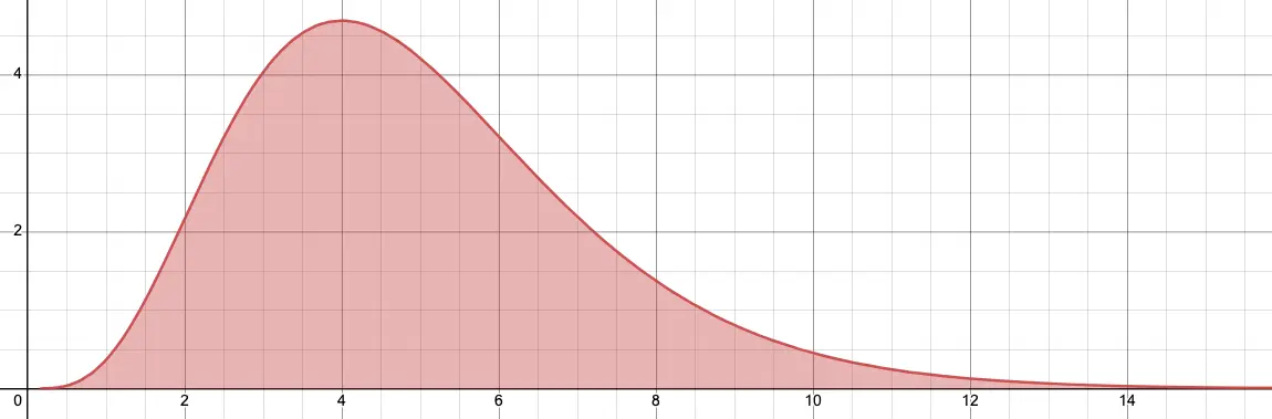
tells us to plot this function for some value xx:

f(t)=txetf(t) = t^x \cdot e^-t

Then, we find the total area under the curve for any positive value of tt. Here’s a picture of the curve for x=4x = 4.

A graph of the function above
A graph of the function described above. Notice how at first, the function flies upward, but it drops significantly after the peak at t = 4.

Almost magically, for a nonnegative value of xx, the integral above spits out the value of x!x!. And it doesn’t stop there. This new definition of x!x! has absolutely no trouble with decimals, complex numbers, irrational numbers, and anything else you can think of. It only has one problem: negative integers.

Well, that was for nothing

No! Don’t click off and start checking (insert name of whatever social media platform is “cool” now)! We’re about to wrap up everything, and we can even fix the problem with negative numbers.

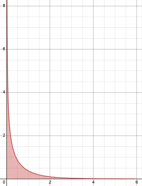
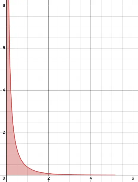
First, I need to explain why the gamma function doesn’t work on negative integers. I’ll start by including two graphs of the function inside the integral
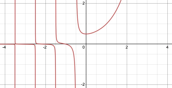
 for x=0.5x = -0.5 and x=1x = -1.

A graph of the function described above at x = 0.5
A graph of the integral for x = 0.5.

A graph of the function described above at x = 1
A graph of the integral for x = 1.

Notice how in the picture where x=0.5x = -0.5, the top and right parts of the function taper to almost nothing, and the only area is in the bottom left. In this case, the function’s area is able to converge, which means it has a value that doesn’t approach infinity.

However, when x=1x = -1, the function has a solid chunk of area on the top-left section, preventing its area from converging on a specific value. In fact, why don’t we just plot this new factorial as a graph?

The gamma function plotted in Desmos

Notice how in the graph, there are reasonable values for the function at any decimal number, but their signs alternate. For a value of xx where 2<x<1-2 < x < -1, x!x! will be negative, and values closer to whole numbers will extend outward to -\infty.

However, for values of xx where 3<x<2-3 < x < -2, x!x! will be positive, and values closer to 3-3 or 2-2 will be “closer” to ++\infty. And that’s the problem.

2-2 is being stretched between two values: it could be -\infty or ++\infty, and we have no way of knowing which, so we just define it, and the factorial of all other negative numbers, to be undefined.

You may think this ends our journey. But there’s one last trick we can use to corral these factorials.

Using limits

Limits are a concept from calculus, which makes them sound scary, but they’re not that difficult. Essentially, limits let us divide by zero and approach infinity without actually getting to that point.

For example, imagine we have this function:

f(x)=x2x6x3f(x) = \frac{x^2 - x - 6}{x - 3}

What is its value at x=2x = 2? It’s just

f(x)=x2x6x3f(2)=222623=4261=41=4\begin{align*} f(x) &= \frac{x^2 - x - 6}{x - 3} \\ f(2) &= \frac{2^2 - 2 - 6}{2 - 3} \\ &= \frac{4 - 2 - 6}{-1} \\ &= \frac{-4}{-1} \\ &= 4 \end{align*}

What about x=1x = 1?

f(x)=x2x6x3f(2)=121613=1162=62=3\begin{align*} f(x) &= \frac{x^2 - x - 6}{x - 3} \\ f(2) &= \frac{1^2 - 1 - 6}{1 - 3} \\ &= \frac{1 - 1 - 6}{-2} \\ &= \frac{-6}{-2} \\ &= 3 \end{align*}

What about x=3x = 3?

f(x)=x2x6x3f(2)=323633=9360=00=undefined\begin{align*} f(x) &= \frac{x^2 - x - 6}{x - 3} \\ f(2) &= \frac{3^2 - 3 - 6}{3 - 3} \\ &= \frac{9 - 3 - 6}{0} \\ &= \frac{0}{0} \\ &= \text{undefined} \end{align*}

We seem to have run into an issue; we’re trying to divide by 00, which is forbidden. Let’s look at the graph of this function and see where we went wrong.

The graph of f of x equals x squared minus x minus 6

Hmm. It looks like our function is a line! Let’s try factoring it.

f(x)=x2x6x3=(x+2)(x3)x3=(x+2)(x3)x3=x+2\begin{align*} f(x) &= \frac{x^2 - x - 6}{x - 3} \\ &= \frac{(x + 2) \cdot (x - 3)}{x - 3} \\ &= \frac{(x + 2) \cdot \cancel{(x - 3)}}{\cancel{x - 3}} \\ &= x + 2 \end{align*}

If our equation is equivalent to x+2x + 2, why does it break at x=3x = 3? Well, we have a denominator of x3x - 3, which for x=3x = 3 evaluates to 33=03 - 3 = 0, and we can’t have a denominator of 00. So our simplified version f(x)=x+2f(x) = x + 2 needs a disclaimer that says xx cannot be 33.

However, limits avoid this problem entirely. They get arbitrarily close to a given point without actually evaluating it at that value. Here’s the function at
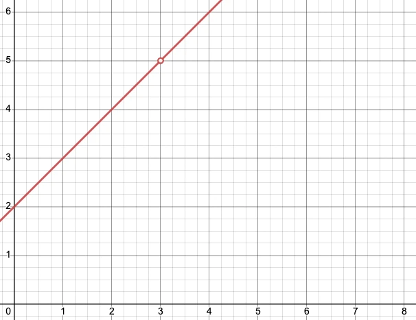
 x=3x = 3, rewritten using limits.

limx3x2x6x3\lim \limits_{x \rarr 3} \frac{x ^ 2 - x - 6}{x - 3}

This expression says, “Evaluate x2x6x3\frac{x ^ 2 - x - 6}{x - 3} with xx as close to 33 as you can get, but not actually at x=3x = 3.” Because x3x \not = 3, we can use the factoring trick and the expression is still valid.

limx3x2x6x3=limx3(x+2)\lim \limits_{x \rarr 3} \frac{x ^ 2 - x - 6}{x - 3} = \lim \limits_{x \rarr 3} (x + 2)

However, limits have another cool property. Inside a limit, we can ignore any restrictions imposed by the original expression, so we can now plug 33 into the right hand side of the limit!

limx3(x+2)=limx35\lim \limits_{x \rarr 3} (x + 2) = \lim \limits_{x \rarr 3} 5

Of course, this expression doesn’t depend on the limiting variable xx anymore, so we can remove the limit and leave the plain value.

limx35=5\lim \limits_{x \rarr 3} 5 = 5

And we’re done! This may not be the actual value of f(x)f(x) at x=3x = 3, but we approximated it using limits and got a pretty reasonable answer. We can do the exact same thing to find the negative cells in Pascal’s Triangle.

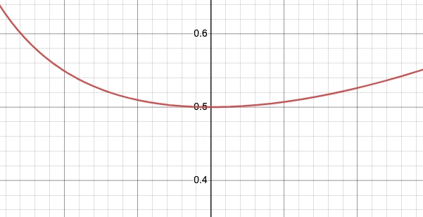
For example, let’s try computing the value of P1,0P_{-1,0}. We already know it should be 0.50.5 from our symmetry experiments, but let’s verify it for sure. Here’s the limit we’re going to compute.

limx0P(1+x),(0+x)=limx0(1+x+0+x)!(1+x)!(0+x)!=limx0(1+2x)!(1+x)!x!\begin{align*} \lim \limits_{x \rarr 0} P_{(-1 + x),(0 + x)} &= \lim \limits_{x \rarr 0} \frac{(-1 + x + 0 + x)!}{(-1 + x)! \cdot (0 + x)!} \\ &= \lim \limits_{x \rarr 0} \frac{(-1 + 2x)!}{(-1 + x)! \cdot x!} \\ \end{align*}

A great way to calculate limits is to prove what the exact value is by spending a fortnight performing intense calculation that will destroy your social life and possibly make you starve.

Another is to graph what you’re limiting.

Let’s do the second option. I’ll plug the limit into Desmos as a function of
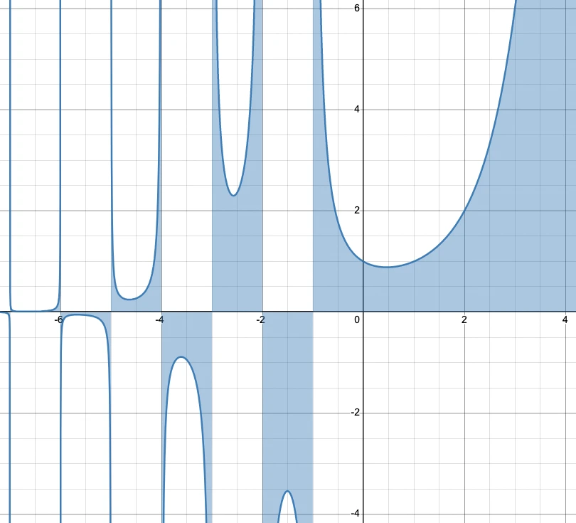
 xx. Here’s the plot.

The function described above

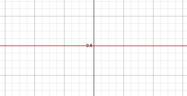
Let’s zoom in a bit.

The same function, zoomed in

Let’s zoom in on the limit, where the curve approaches a straight line.

The same function, zoomed in

It looks like we get y=0.5y = 0.5, which is exactly what we predicted! In fact, we can get any other value in Pascal’s Triangle just by taking different limits. Here are the results of every value from P6,5P_{-6,-5} to P4,3P_{4,3}.

000000.52.555000000.5232000000.51.51.50.5000000.510.50000000.50.500000000.50000.50.50.50.50.5111121.510.50123431.50.5001361020.50001410200.5000015153500000162156\begin{matrix} 0 & 0 & 0 & 0 & 0 & 0.5 & -2.5 & 5 & -5 \\ 0 & 0 & 0 & 0 & 0 & 0.5 & -2 & 3 & -2 \\ 0 & 0 & 0 & 0 & 0 & 0.5 & -1.5 & 1.5 & -0.5 \\ 0 & 0 & 0 & 0 & 0 & 0.5 & -1 & 0.5 & 0 \\ 0 & 0 & 0 & 0 & 0 & 0.5 & -0.5 & 0 & 0 \\ 0 & 0 & 0 & 0 & 0 & 0.5 & 0 & 0 & 0 \\ 0.5 & 0.5 & 0.5 & 0.5 & 0.5 & 1 & 1 & 1 & 1 \\ -2 & -1.5 & -1 & -0.5 & 0 & 1 & 2 & 3 & 4 \\ 3 & 1.5 & 0.5 & 0 & 0 & 1 & 3 & 6 & 10 \\ -2 & -0.5 & 0 & 0 & 0 & 1 & 4 & 10 & 20 \\ 0.5 & 0 & 0 & 0 & 0 & 1 & 5 & 15 & 35 \\ 0 & 0 & 0 & 0 & 0 & 1 & 6 & 21 & 56 \\ \end{matrix}

There are a lot of patterns in this shape.

The easy one to spot is the quadrant of zeroes in the top-left. Specifically, if both the row number aa and the column number bb are less than 00, the cell’s value will be 00.

There are two other fields of zeroes that are shaped like triangles: one at the bottom-left of the square, and one at the top-right. Do you remember the formulas we found on a per-column basis? Here’s an example of one:

(n+1)(n+2)(n+3)(n+4)4!\frac{(n + 1) (n + 2) (n + 3) (n + 4)}{4!}

This formula corresponds to the fourth row or column. That row has 4 zeroes because if nn is 1-1, then the n+1n + 1 term is zero and the entire formula goes to 00. Similarly, nn could be 2-2, in which case n+2n + 2 would be zero, 3-3, or 4-4.

There are more patterns. The rows and columns of 0.50.5 and 11 are very noticeable. The 11s result from how we define Pascal’s Triangle, and the 0.50.5s eventually combine to make the long trail of 11s.

Additionally, every column in the top-right section either has only positive numbers or only negative numbers. This excludes the number in the bottom-right quadrant. To make it clearer, I’ll highlight one of these columns.

000000.52.555000000.5232000000.51.51.50.5000000.510.50000000.50.500000000.50000.50.50.50.50.5111121.510.50123431.50.5001361020.50001410200.5000015153500000162156\begin{matrix} 0 & 0 & 0 & 0 & 0 & 0.5 & \boxed{-2.5} & 5 & -5 \\ 0 & 0 & 0 & 0 & 0 & 0.5 & \boxed{-2} & 3 & -2 \\ 0 & 0 & 0 & 0 & 0 & 0.5 & \boxed{-1.5} & 1.5 & -0.5 \\ 0 & 0 & 0 & 0 & 0 & 0.5 & \boxed{-1} & 0.5 & 0 \\ 0 & 0 & 0 & 0 & 0 & 0.5 & \boxed{-0.5} & 0 & 0 \\ 0 & 0 & 0 & 0 & 0 & 0.5 & 0 & 0 & 0 \\ 0.5 & 0.5 & 0.5 & 0.5 & 0.5 & 1 & 1 & 1 & 1 \\ -2 & -1.5 & -1 & -0.5 & 0 & 1 & 2 & 3 & 4 \\ 3 & 1.5 & 0.5 & 0 & 0 & 1 & 3 & 6 & 10 \\ -2 & -0.5 & 0 & 0 & 0 & 1 & 4 & 10 & 20 \\ 0.5 & 0 & 0 & 0 & 0 & 1 & 5 & 15 & 35 \\ 0 & 0 & 0 & 0 & 0 & 1 & 6 & 21 & 56 \\ \end{matrix}

The same pattern occurs in the bottom-left corner, but with rows of same-sign numbers instead of columns.

000000.52.555000000.5232000000.51.51.50.5000000.510.50000000.50.500000000.50000.50.50.50.50.5111121.510.50123431.50.5001361020.50001410200.5000015153500000162156\begin{matrix} 0 & 0 & 0 & 0 & 0 & 0.5 & -2.5 & 5 & -5 \\ 0 & 0 & 0 & 0 & 0 & 0.5 & -2 & 3 & -2 \\ 0 & 0 & 0 & 0 & 0 & 0.5 & -1.5 & 1.5 & -0.5 \\ 0 & 0 & 0 & 0 & 0 & 0.5 & -1 & 0.5 & 0 \\ 0 & 0 & 0 & 0 & 0 & 0.5 & -0.5 & 0 & 0 \\ 0 & 0 & 0 & 0 & 0 & 0.5 & 0 & 0 & 0 \\ 0.5 & 0.5 & 0.5 & 0.5 & 0.5 & 1 & 1 & 1 & 1 \\ -2 & -1.5 & -1 & -0.5 & 0 & 1 & 2 & 3 & 4 \\ \boxed{3} & \boxed{1.5} & \boxed{0.5} & 0 & 0 & 1 & 3 & 6 & 10 \\ -2 & -0.5 & 0 & 0 & 0 & 1 & 4 & 10 & 20 \\ 0.5 & 0 & 0 & 0 & 0 & 1 & 5 & 15 & 35 \\ 0 & 0 & 0 & 0 & 0 & 1 & 6 & 21 & 56 \\ \end{matrix}

Conclusion and challenges

Well, that was fun! I hope you liked reading this article as much as I did while writing it. Whether you’re an advanced mathematician or a regular person, you will definitely have learned something about math and Pascal’s Triangle today.

If you really liked this article, you can subscribe to the zSnout blog by creating a zSnout account. If you don’t want to get notified, don’t worry! Just log in, head to the list of blog articles, and disable notifications from there.

For those of you who are looking for more to do with Pascal’s Triangle, here are some ideas to explore:

  • Pascal’s Pyramid: You can extend Pascal’s Triangle into 3 dimensions, creating an analog known as Pascal’s Pyramid. Find out how to modify our formula to work in 3 dimensions and explore its applications.

  • Decimals: The gamma function, and consequently, our formula, works perfectly fine on decimals. Explore how Pascal’s Triangle would work with decimal coordinates.

  • Graphing: Once you’ve figured out what decimal input to our formula means, plot our formula in 3 dimensions as a function z=(x+y)!x!y!z = \frac{(x + y)!}{x! \cdot y!} and explore the patterns you get.

  • Complex numbers: Plug complex numbers into our formula and find a pattern in the outputs. Disclaimer: you may need to be a 6 or 7 dimensional being to observe the full pattern.

Thanks for reading this blog article on zSnout! Stay tuned for next week, where we’ll be visiting the Saurs on their home planet.

References

”3D Calculator - GeoGebra.” GeoGebra, 23 Nov. 2022, https://www.geogebra.org/calculator.

  • I used GeoGebra’s 3D calculator to explore the plot of the formula z=(x+y)!x!y!z = \frac{(x + y)!}{x! \cdot y!} as a 3 dimensional graph.

”Gamma function - Wikipedia.” Wikipedia, 22 Nov. 2022, https://en.wikipedia.org/wiki/Gamma_function.

  • I checked this article to find the relationship between Γ(x)\Gamma(x) and x!x! after I forgot everything from “How to Take the Factorial of Any Number."

"How to Take the Factorial of Any Number.” YouTube, uploaded by Lines That Connect, 22 Nov. 2022, https://www.youtube.com/watch?v=v_HeaeUUOnc&t=1329s.

  • This is a very interesting video about how to extend the factorial function.
  • It was my “formal” introduction to analytically continuing a sequence.
  • It also explains the history of the gamma function concisely.

”Limits intro (article) | Khan Academy.” Khan Academy, 23 Nov. 2022, https://www.khanacademy.org/math/ap-calculus-ab/ab-limits-new/ab-1-2/a/limits-intro.

  • I copied this article’s formula about a function that requires a limit to be evaluated.

”Pascal’s pyramid.” Wikipedia, 23 Nov. 2022, https://en.wikipedia.org/wiki/Pascal%27s_pyramid.

  • This article explores the mathematical properties of Pascal’s Pyramid.
  • This was my first introduction to a higher dimensional version of Pascal’s Triangle.

”Wolfram|Alpha: Computational Intelligence.” Wolfram|Alpha, 23 Nov. 2022, https://www.wolframalpha.com/.

  • I used Wolfram|Alpha to evaluate the limits after manually adding .9999.9999\dots to evaluate limits in Desmos got tiring.

Zachary Sakowitz. “Extended Factorial Function.” Desmos, 23 Nov. 2022, https://www.desmos.com/calculator/pd4wbpvxfc.

  • I used this Desmos graph as an image in this article.

Zachary Sakowitz. “Pascal’s Pyramid.” Desmos, 23 Nov. 2022, https://www.desmos.com/calculator/qwl9nfuw5k.

  • This graph is the remnants of my brief exploration of Pascal’s Pyramid.

Zachary Sakowitz. “Pascal’s Triangle.” Desmos, 23 Nov. 2022, https://www.desmos.com/calculator/xk1nk7ewrx.

  • This graph helped me to first see the patterns in the negative regions of Pascal’s Triangle before I was able to prove them with calculus.

”Zeros and poles - Wikipedia.” Wikipedia, 22 Nov. 2022, https://en.wikipedia.org/wiki/Zeros_and_poles.